Stock Market Timing Using P/E SMA Signals

A subscriber proposed four alternative ways of timing the U.S. stock market based on simple moving averages (SMA) of the market price-earnings ratio (P/E), as follows:

1. 5-Year Binary – hold stocks (cash) when P/E is below (above) its 5-year SMA.
2. 10-Year Binary – hold stocks (cash) when P/E is below (above) its 10-year SMA.
3. 15-Year Binary – hold stocks (cash) when P/E is below (above) its 15-year SMA.
4. 5-Year Scaled – hold 100% stocks (cash) when P/E is five or more units below (above) its 5-year SMA. Between these levels, scale allocations linearly.

To obtain a sample long enough for testing these rules, we use the monthly U.S. data of Robert Shiller. While offering a very long history, this source has the disadvantage of blurring monthly data as averages of daily values. How well do these alternative timing strategies work for this dataset? Using monthly data for the S&P Composite Index, annual dividends, annual P/E and 10-year government bond yield since January 1871 and monthly 3-month U.S. Treasury bill (T-bill) yield as return on cash since January 1934, all through August 2018, we find that:

Assumptions for testing are:

• There is a 6-month delay in availability of P/E data due to the earnings release/revision process.
• Total monthly S&P 500 Composite Index return is the capital gain plus one twelfth of the annual dividend yield recorded for that month.
• Return on cash is the T-bill yield after 1933. Return on cash prior to 1934 is the Shiller 10-year government bond yield minus the post-1933 average term spread (bond yield minus T-bill yield).
• Switching between/rebalancing the stock index and cash and reinvestment of dividends are frictionless.

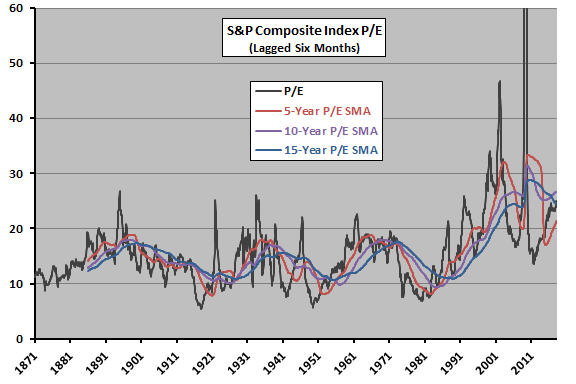
The following chart tracks S&P Composite Index P/E and the three specified P/E SMAs, lagged by six months as assumed, over the available sample period. The vertical axis is truncated at 60 for visibility. Lagged values are higher than 60 during nine months from July 2009 through March 2010.

How do the specified SMA rules translate to market timing performance?

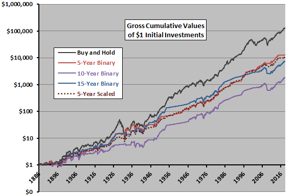
The next chart compares gross cumulative values of buy-and-hold and the four market timing strategies starting in 1886 (to enable calculation of an initial 15-year SMA). Buy-and-hold prevails based on terminal value/compound annual growth rate (CAGR). The sample is not long in terms of number of independent SMA calculation intervals, so the timing cumulatives are noisy. It appears the 10-Year Binary strategy is unlucky compared to the 5-Year and 15-Year Binary strategies. The 5-Year Scaled strategy performs similarly to the 5-Year Binary strategy, with lower volatility.

For additional insight, we look at an array of performance statistics.

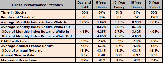
The following table summarizes gross overall, monthly and annual performance statistics for buy-and-hold and all four stock market timing strategies, with notable points as follows:

• All four timing strategies produce an average allocation to the stock market index of about 50%.
• The 5-Year, 10-Year and 15-Year Binary strategies switch between the stock market index and cash an average of once every 1.3, 2.0 and 2.5 years, respectively. The 5-Year Scaled strategy requires rebalancing in 80% of all months.
• The average monthly total return for the S&P Composite Index is notably higher when the 5-Year and 15-Year Binary strategies are in stocks than when they are out of stocks, but the opposite is true for the (unlucky) 10-Year Binary strategy. This conflict undermines confidence in the timing approach. (The average monthly total return for the 5-Year Scaled strategy includes both the stock market index and cash allocations.)
• Buy-and-hold easily beats the timing strategies based on CAGR and average annual total return in excess of the risk-free rate (same as the return on cash).
• The timing strategies, especially, 5-Year Scaled, exhibit much lower annual volatilities than buy-and-hold, such that 5-Year Binary and especially 5-Year Scaled are competitive (on a gross basis) with buy-and-hold based on Sharpe ratio.
• All timing strategies, again especially 5-Year Scaled, substantially suppress maximum drawdown compared to buy-and-hold.

Accounting for switching/rebalancing frictions would materially reduce performance of the timing strategies, especially 5-Year Scaled, relative to buy-and-hold.

Results are generally robust to assuming no delay or a delay less than six months in availability of monthly P/E values.

In summary, evidence from a long conceptual test indicates that U.S. stock market timing based on P/E moving averages may have some attractive aspects for risk-averse investors, but this approach does not keep up with buy-and-hold.

Cautions regarding findings include:

• Relying strictly on stock market index P/E ignores any yield competition between equities and other asset classes.
• As noted, input data is blurred by calculating monthly levels as averages of daily values during each month. Results for end-of-month data may differ.
• As noted, results are gross, not net. Accounting for costs of switching between stocks and cash would lower returns. For the 5-Year Scaled strategy, there are rebalancing costs most months. Such costs are likely material during much of the sample period. Had current low costs (and tax-deferred retirement accounts) been in existence across the sample period, market behaviors might well have been different.
• Use of an index rather than a tradable asset to calculate returns ignores the costs of maintaining a liquid fund. These costs would reduce returns and are likely material during much of the sample period.
• The assumed 6-month lag in availability of P/E data may be overly conservative. However, results are similar for a 3-month lag and no lag.
• The approach to estimating the risk-free rate prior to 1934 impounds look-ahead bias. Also, term spread drivers may have been different before 1934.

See also “Usefulness of P/E10 as Stock Market Return Predictor” and “Alternative Tests of P/E10 Usefulness”.