Are there exploitable lead-lag relationships between bonds and stocks, perhaps because bond investors are generally better informed than stock investors or because there is some predictable stocks-bonds rebalancing cycle? To investigate, we examine lead-lag relationships between bond exchange-traded fund (ETF) returns and stock ETF returns. We consider iShares iBoxx $ Investment Grade Corporate Bond (LQD) and iShares iBoxx $ High-Yield Corporate Bond (HYG) as liquid bond ETFs and SPDR S&P 500 (SPY) as a liquid stock ETF. Using dividend-adjusted daily, weekly and monthly returns for LQD, HYG and SPY during mid-April 2007 (HYG inception) through March 2018, we find that:
For all three measurement frequencies, average HYG and LQD returns are similar, and lower than average SPY return. LQD volatility is lower than that of HYG, and both bond fund volatilities are lower than that of SPY.
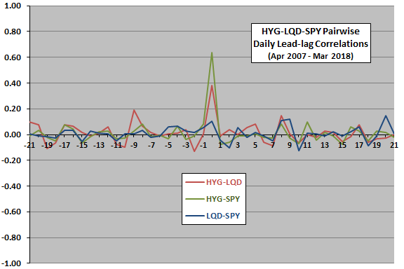
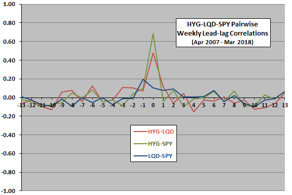
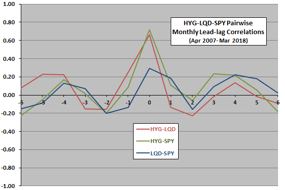
The following three charts plot pairwise lead-lag relationships at daily (upper chart), weekly (middle chart) and monthly (lower chart) frequencies. For each pair, correlations summarize lead-lag relationships ranging from first pair member return leads second pair member return by 21 days (-21 in upper chart), 13 weeks (-13 in middle chart) or six months (-6 in lower chart) to second pair member return leads first pair member return by 21 days (21 in upper chart), 13 weeks (13 in middle chart) or six months (6 in lower chart).
For example, in the upper chart, the value for the blue line at -1 is the correlation for SPY return leading LQD return by one month, and the value for the blue line at 1 is the correlation for LQD return leading SPY return by one month.
In general, relationships appear unexploitably coincident (correlation peaks are at 0, and other correlations may be just noise). However, we check further on: (1) the indication in the middle chart that SPY return leads LQD return by one week; and, (2) the indication in the lower chart that LQD return leads SPY return by one month. Specifically, we check robustness versus noise by looking at subperiods.
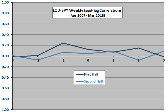
The next two charts summarize correlations for:
Upper chart: weekly lead-lag relationships between LQD and SPY ranging from SPY return leads LQD return by three weeks (-3) to LQD return leads SPY return by three weeks (3) during two equal subperiods.
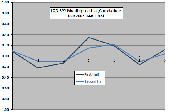
Lower chart: monthly lead-lag relationships between LQD and SPY ranging from SPY return leads LQD return by three months (-3) to LQD return leads SPY return by three months (3) during two equal subperiods.
The break point for subperiods is October 2012. Results suggest the finding that LQD return leads SPY return by one month is the more reliable of the two indications. To check for linearity in this relationship, we look at average next-month SPY performance across ranges of monthly LQD returns.
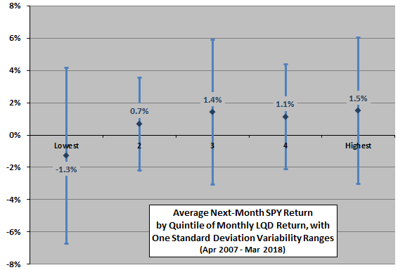
The next chart summarizes average next-month SPY return by ranked fifth (quintile) of monthly LQD return. Results suggest a left-tail effect, with very weak monthly LQD return indicating relatively weak next-month SPY return but probably no exploitable findings across other quintiles.
To quantify the economic value of this finding, we look at a strategy that simply avoids stocks after unusually bad months for LQD.
Assumptions for the strategy are:
- Each month hold SPY (cash) when prior-month LQD return is above (below) either 0% or -1%, designated Timed SPY (0%) and Timed SPY (-1%), respectively.
- It is feasible to anticipate LQD monthly returns slightly, such that signals and signaled switches occur at the same monthly closes.
- SPY-cash switching frictions are 0.1% of traded value.
- Return on cash is zero (close to true over the available sample period), to the advantage of buying and holding SPY.
- Ignore tax implications of trading.
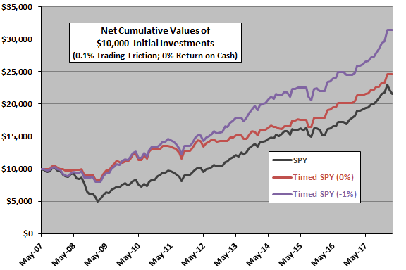
The final chart compares net cumulative values of $10,000 initial investments in SPY, Timed SPY (0%) and Timed SPY (-1%) over the available sample period. Net compound annual growth rates for SPY, Timed SPY (0%) and Timed SPY (-1%) are 7.3%, 8.6% and 11.1%, respectively. Maximum drawdowns are -51%, -21% and -22%, respectively (all during 2008-2009). The advantage of timing comes largely during the 2008-2009 equity market crash.
Timed SPY (0%) and Timed SPY (-1%) switch between SPY and cash 66 and 32 times, respectively, and are in SPY 61% and 81% of the time. The latter is therefore less sensitive to level of trading frictions.
In summary, evidence from simple tests suggests that LQD may lead SPY exploitably at a monthly frequency.
Cautions regarding findings include:
- Most of the above tests are in-sample. An investor operating in real time based only on these data would not know to follow the strategy.
- The sample period is short for a monthly strategy, and includes a dominating event (the 2008-2009 crash) that strongly affects outcome. This caution seems common to many intermediate-term timing strategies tested with recent ETF data.
- ETF dividend cycles may influence correlations.
- Testing different pairs, different measurement frequencies and (in the final test) different signal thresholds introduces data snooping bias, such that results for the best parameter settings overstate expectations. Having an extreme event in the sample can amplify this bias.
See also the much longer-term, more qualitative assessment in “Bonds Lead Stocks?”.