“Trend Factor and Stock Returns” describes a method of extracting information from stock price simple moving averages (SMA) that is more complicated than that used by most traders. Instead of using current price above or below an SMA as a signal, this method employs offset regressions (normalized SMAs lagged one month behind returns) to project next month’s return based on current SMAs. Does this alternative use of SMAs usefully forecast stock market returns. To investigate, we apply the methodology to predict SPDR S&P 500 (SPY) returns and to predict International Business Machines Corporation (IBM) returns. Using daily dividend-adjusted closes for SPY since the end of January 1993 and for IBM since the beginning of January 1962, both through November 2012, we find that:
First, for SPY, at the end of each month we:
- Calculate SPY SMAs for the past 3, 5, 10, 20, 50, 100 and 200 trading days.
- Normalize the SMAs by dividing by the final SPY close.
- Regress monthly normalized SMAs against next-month SPY returns over the past one to four years to estimate the relationship between normalized SMAs and next-month SPY return.
- Use the current normalized SMAs to forecast SPY return for the next month (via the Excel FORECAST function).
- Calculate a composite forecast by averaging the individual forecasts for all seven SMAs.
We then test the abilities of the forecast average and individual SMA forecasts to predict monthly SPY returns. Results optimistically assume that an investor can accurately perform calculations just before the monthly close and execute at the same close.
Note that this approach deviates (for simplicity) from that in the referenced study, which uses multiple regressions, rather than averages of single regression outputs, to combine the effects of different SMAs. Use of single regressions assumes that the individual SMAs contribute equally to aggregate predictive power.
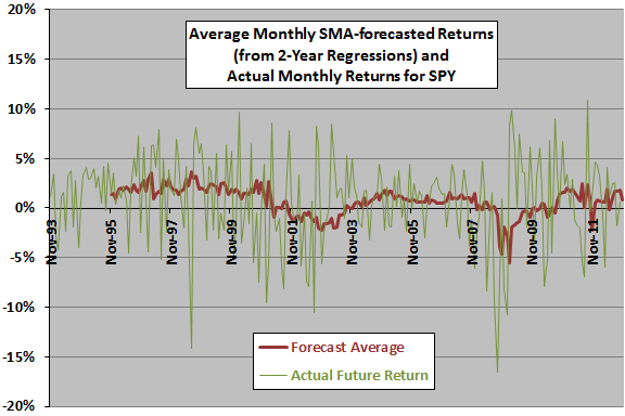
The following chart shows the monthly average forecasted SPY return from two-year lagged regressions of all seven SMAs and actual monthly returns for SPY over the available sample period. It appears that there may be some relationship between forecasts and actuals, but forecasts may lag actuals (as expected for SMA and regression calculations).
Why use a two-year regression interval?
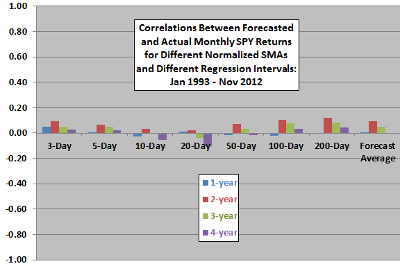
The next chart summarizes correlations between forecasted and actual monthly SPY returns for each of the seven SMAs and for the average based on lagged regression intervals of one to four years, over the available sample period. In general, a two-year regression interval generates the strongest agreement between forecasts and actuals. However, correlations are generally small and inconsistent across regression intervals, varying in magnitude and sign. Results undermine belief in a stable predictive power for normalized SMAs.
Note that in-sample selection of the two-year regression interval introduces data snooping bias, such that results likely overstate future predictive power.
Might there be an important non-linearity in the relationship?
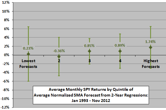
The next chart summarizes average actual monthly SPY returns, with one standard deviation variability ranges, for months sorted into fifths (quintiles) of the forecast average across all SMAs. Based on average return, the progression is nearly systematic across quintiles. On a volatility-adjusted basis (average divided by standard deviation), quintile 5 is best (0.36), followed by quintiles 3, 4, 1 and 2.
This analysis is in-sample. An investor operating in real time would have only past data (not the entire sample) to estimate when forecasted returns are relatively high or low. Limiting inputs to real-time data may change results.
Might this approach work better on an individual stock?
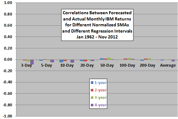
The next chart summarizes correlations between forecasted and actual monthly IBM returns for each of the seven SMAs and for the average based on lagged regression intervals of one to four years, over the available sample period. Correlations are generally smaller than for SPY and still inconsistent across regression intervals, undermining belief in a stable predictive power for normalized SMAs.
Might there be an important non-linearity here?
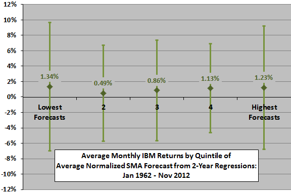
The final chart summarizes average actual monthly IBM returns, with one standard deviation variability ranges, for months sorted into quintiles of the forecast average across all SMAs. Based on average return, the progression is systematic except for quintile 1. On a volatility-adjusted basis, results are less systematic, with quintile 4 best (0.20), followed by quintiles 1, 5, 3 and 2. The relatively strong performance of quintile 1 likely derives from the inability of SMAs and regressions to identify turning points (rebounds from crashes).
Again, this analysis is in-sample. An investor operating in real time would have only past data to estimate when forecasted returns are relatively high or low. Limiting inputs to real-time data may change results.
In summary, evidence from simple tests offers some support a belief that normalized SMA regressions usefully predict stock returns.
Cautions regarding findings include:
- In general, linear regression analysis assumes a linear relationship between dependent and independent variables and normal distributions for variables.
- As noted, most of the above tests are in-sample, and selection of the two-year regression for SPY return forecasts incorporates data snooping bias. The sensitivity of findings to the length of the regression interval is a strong concern.
- Realistic trading strategies with frictions would underperform any findings above.